CSE 168 Final Project
Transmission
I implemented transmission using the GGX microfacet model1. The relevant command is transmission. Note that there is no specific ior command because the index of refraction is actually automatically determined from the specular value, according to Schlick’s approximation2. Essentially, the value given in specular is the color seen when directly looking at the object, which allows us to solve for the index of refraction . For example, glass has the index of refraction . Using Schlick’s approximation, this roughly translates to a specular value .
In order to conserve energy, I have the following setup: first calculate the amount of specular reflection (e.g. the Fresnel term ), and then take to be the remaining amount. This is then distributed among diffusion and transmission. Therefore diffuse and transmittance actually represent the percentage of the remaining energy that is diffused/transmitted. As long as diffuse + transmittance <= 1 and specular <= 1, energy does not increase. This setup is a little awkward, but it works well enough.
Also, I did not use Schlick’s approximation to compute , despite using it to approximate . When it came time to actually compute , I instead went with the full formula described in the GGX paper1. Originally I had not planned to do so, but there is a reason for this: Schlick’s approximation does not account for total internal reflection (TIR). It always interpolates over the full interval , rather than maxing out at an earlier . However, how TIR actually works is that we should see a smooth fade between the refraction and reflection terms. At the TIR critical angle, there should not be a sharp visual effect caused by suddenly discarding invalid rays, because we should have before that point.
Update: 6/12/2024
I realize this comes after the due date, so feel free to ignore the following section. I just thought the issue with Schlick’s approximation deserved a better explanation.
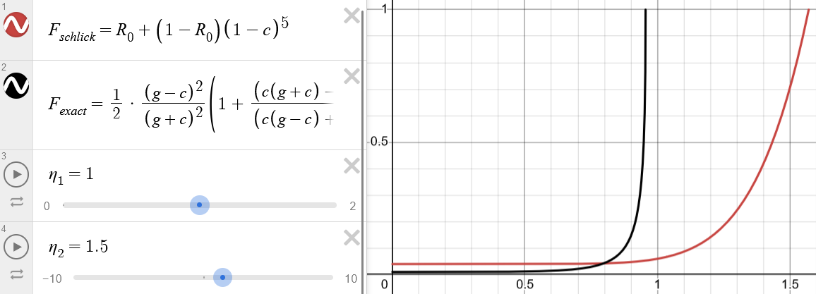
The easiest way to see how Schlick’s approximation does not handle TIR is that it does not distinguish between which index of refraction ( or ) corresponds to the entered/exited medium. Schlick’s approximation is symmetric in that respect. However, the exact formula is not symmetric. Let be the entered medium and be the exited medium. Schlick’s approximation is only accurate when .
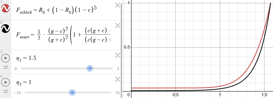
 vs. : Red is Schlick’s approximation, and black is the exact formula. and are chosen to represent glass and air. Technically, , but I have chosen for my program.
Anyway, enough of the discussion on implementation. I think the following image best illustrates my implementation of transmission. I repurposed the GGX test scene from Homework 4.
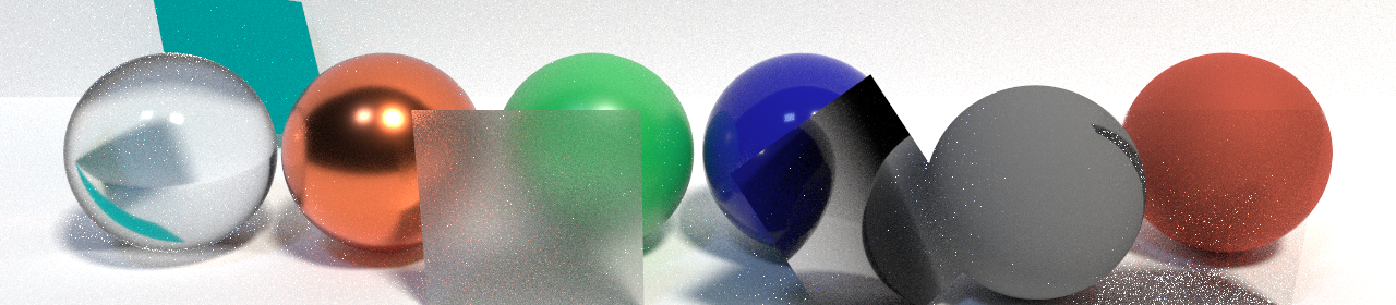 GGX spheres and planes: The sphere on the left has
 specular 0.04 0.04 0.04, the plane on the middle-left has roughness 0.3, the plane on the middle-right is experiencing TIR (the black color is due to there being no sky), and the plane on the right has specular 0.00001 0.00001 0.00001 and is almost fully transparent. This scene was rendered with MIS at 2048spp.
Note that the planes in the above image are bending light, which doesn’t make much physical sense (refraction should be barely noticeable for thin mediums). The program checks to determine if light is entering/exiting a medium. If incoming light is aligned with the normal, it is treated as entering a medium. And if incoming light is not aligned with the normal, then it is treated as exiting a medium. So in order to be physically accurate, all objects must have front and back facing geometry. For demonstration purposes, these planes do not, which is why the refraction is noticeable. The plane on the middle-left is facing towards the camera (the camera’s perspective is from the “exterior”), while the plane on the middle-right is facing away from the camera (the camera’s perspective is from the “interior,” which is why we see TIR).
Depth of Field
Depth of field is quite simple to achieve. With path tracing, it is essentially a free feature. All that needs to be done is for the ray origins to be perturbed by some small amount while fixing points at a specific distance, called the “subject distance” (okay, it’s slightly more complicated than that, but it really is quite simple). The relevant commands here are aperture and subjectdistance. In photography, aperture is often described with an “f-number,” but the aperture command instead refers to relative aperture. Relative aperture is simply the reciprocal of the f-number (e.g. aperture 0.125 is equivalent to f/8).
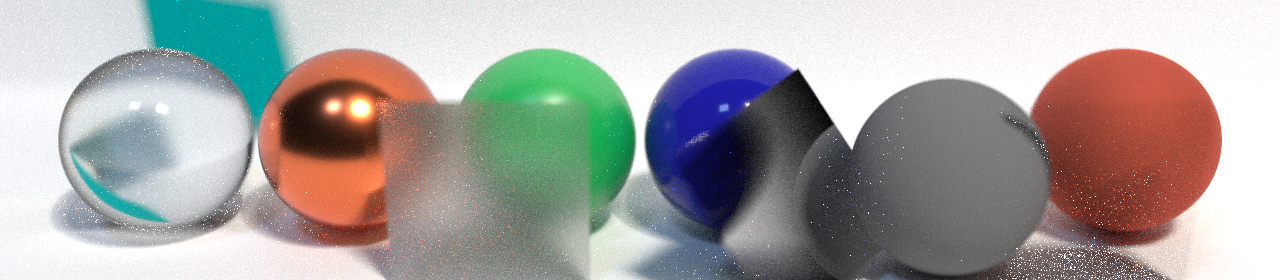 GGX spheres and planes: Same as above, except with
 subjectdistance 13 and aperture 3. Note that the DOF effect occurs for the “interior” of the glass ball (e.g. everywhere but the edges). This is because the light coming through the ball is coming from far away, past the range of clarity.
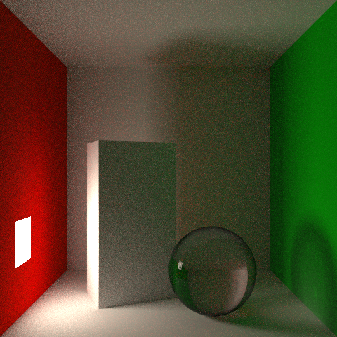
 Cornell box: Another simple demonstration of the DOF effect.
 subjectdistance 2.75, aperture 0.7. I think I may have set the aperture too high, because it was a little hard to get the sphere in focus. To be fair, it’s a little difficult to edit a scene through a text file.
Photon Mapping
Finally, I attempted to implement photon mapping3. However, I decided against fully committing to photon mapping: instead, I only created the caustics photon map. This is because I felt that global illumination was already done quite well by NEE/MIS. On the other hand, caustics look truly horrifying without thousands of samples.
In my implementation, using the photon map is a little cumbersome. Since photon maps can be reused, there is a separate command sampler photon and shader herophoton (it’s called herophoton because the actual shader is called hero). This makes the next render output a photon map (.photons file) instead of an image. To set the number of photons, we reuse the size <x> <y> command, where x * y photons are shot out (it doesn’t really matter that it’s a 2d size parameter; it’s just a relic from reusing commands). Afterwards, we have to switch back to sampler basic and shader hero to render the scene. By default it will ignore the photon map. To make it load/use the photon map, we need to use photonmap <radius> <count> with nonzero values. <radius> controls the maximum search radius for photons, and <count> controls the maximum number of photons to count.
The photons are stored in a -d tree written from scratch, since it’s honestly easier to write one yourself than to take some open-source library. Most online C++ implementations seem to use a linked-node approach, which is really annoying to copy to device memory. My -d tree was flat, which is also more performant. Here are some preliminary results showing the locations of photons in the scene:
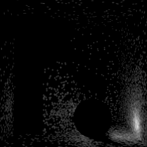 Cornell box: The locations/counts of photons in the scene, with 1,000,000 photons. Keep in mind that there are far fewer than 1,000,000 photons here because the vast majority of them were not for caustics and were therefore discarded.
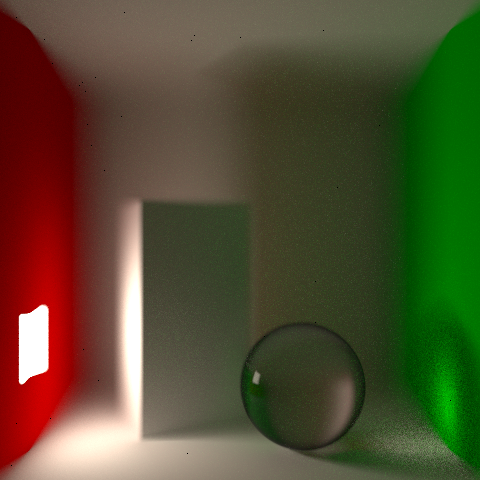
Finally, here is an actual render using the photon map:
 Cornell box: Again, 1,000,000 photons with
 photonmap 0.1 256, nexteventestimation mis, spp 64. The caustics do look quite clean despite a low number of samples.
And here is the ground truth, rendered with brute force (MIS and 2000+ samples per pixel):
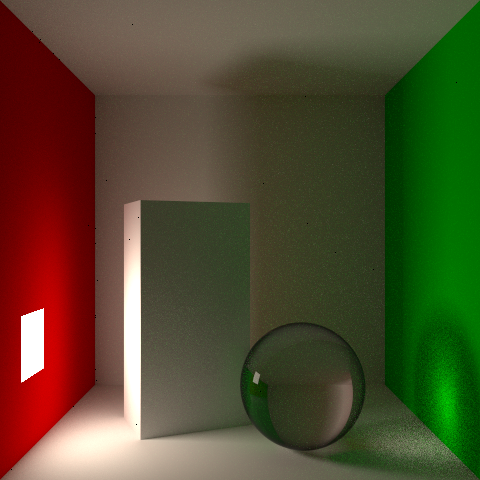 Cornell box: Ground truth.
 nexteventestimation mis, spp 2048.
The caustics do look comparatively clean, but they are evidently wrong. I haven’t quite figured out why yet. It’s a bit sad, but at least it wasn’t a complete failure. :/
My best guess is that I have calculated the power of the photons incorrectly, e.g. in BSDF evaluation. I say this because the shape of the caustics actually match up very closely between the photon-mapped image and the ground truth. My other reason for thinking my BSDF evaluation could be wrong is that when viewing the raw photon count (e.g. in the first image), we do see a higher concentration of photons at the center of the caustic. This indicates to me that my importance sampling is working correctly. I think the lack of a bright spot despite the much higher concentration of photons means that these photons are severely under-powered.
References
-
Bruce Walter, Stephen R Marschner, Hongsong Li, and Kenneth E Torrance. 2007. Microfacet Models for Refraction through Rough Surfaces. In Proceedings of the 18th Eurographics conference on Rendering Techniques. 195–206. https://www.cs.cornell.edu/~srm/publications/EGSR07-btdf.html. ↩ ↩2
-
Henrik Wann Jensen. 2001. Realistic Image Synthesis Using Photon Mapping. A. K. Peters, Ltd., USA. http://graphics.ucsd.edu/~henrik/papers/book/. ↩